Introduction
Flow.bio Documentation
Welcome to Flow.bio, the comprehensive bioinformatics data management platform and open database that makes analyzing biological data accessible to everyone.
Whether you're a wet lab scientist running your first RNA-seq analysis or a bioinformatician managing complex workflows, Flow.bio provides the tools you need to go from raw data to biological insights.
What can you do with Flow?
Flow streamlines the entire bioinformatics data life cycle:
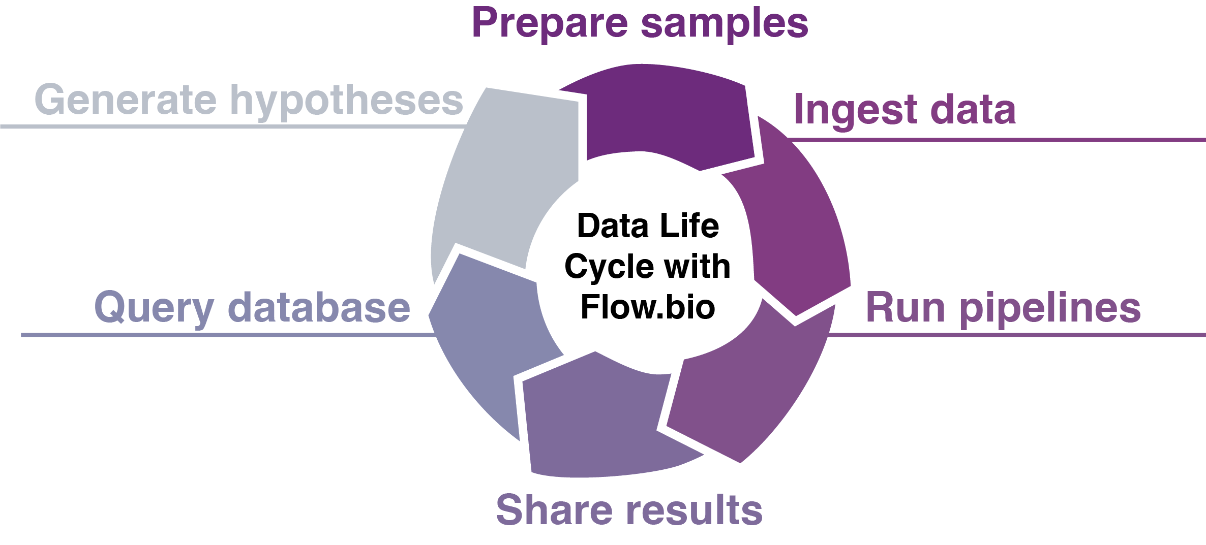
- Upload and organize your sequencing data samples with extensive metadata set by admins
- Run validated Nextflow pipelines for RNA-seq, ChIP-seq, CLIP-seq, and easily add your own
- Visualize results with interactive reports and quality metrics
- Collaborate seamlessly with your team and the scientific community
- Ensure reproducibility with version-controlled pipelines and tracked parameters
- Query the database via the web app or programmatically with our API endpoints.
Getting Started
Create an account
Learn to set up and manage your account
Manage projects
Organise your data into projects and manage permissions
Run pipelines
Analyse your data using curated, validated pipelines
Search data
Find relevant data in our public database
Need Help?
- Check our FAQ for common questions
- Contact support@flow.bio for anything else